Author: David Masad
Source: http://davidmasad.com/blog/ergms-from-scratch/
Exponential random graph models (ERGMs) are statistical models for explaining the structure of social and other networks (also called graphs). If we have a network, and some hypotheses about the factors that make it looks the way it does, an ERGM is meant to tell us how big a role (if any) these factors actually play.
I think of it as a regression model: we have several independent variables we think determine the dependent variable, and the model estimates the size and significance of the effect of each.
For someone like me who works a lot with networks, ERGMs can be a very powerful tool. There is even an excellent R package called, appropriately enough, ergm, that makes estimating ERGMs just about as easy as specifying a regression formula.
I’ve always felt a bit nervous about using them, though, because I didn’t feel confident I really understood how they worked, and how they were being estimated.
Toy ERGM from Scratch
To help with that, I decided I needed to implement a simple toy ERGM from scratch. It didn’t need to be fast, or really applicable at all. The most important thing was to take the methodology apart and put it back together again.
In this post, I’m going to walk through my implementation of a highly simplified ERGM estimation, using Python and the NetworkX package. I’m hoping that it will help others with similar questions, and that people who know more than I do will point out anything I’m getting wrong.
import random
import numpy as np
import networkx as nx
%matplotlib inline
import matplotlib.pyplot as plt
import matplotlib
Graph probabilities
The basic idea of ERGMs is to define a probability distribution over all possible graphs of a given number of nodes, where the probability of each graph is proportional to some of its network statistics. In this post, the statistics I’ll use throughout are the edge count and the number of triangles, but any network statistics will do. If edge count and triangles have coefficients a and b, then the probability of observing a particular graph G is:
\[Pr(G)∝a∗edges(G)+b∗triangles(G)\]or more specifically:
\[Pr(G)∝e^{a∗edges(G)+b∗triangles(G)}\](hence the exponential).
Think of this as the ‘weight’ we put on a particular network. In Python, this looks like:
def compute_weight(G, edge_coeff, tri_coeff):
    '''
    Compute the probability weight on graph G
    '''
    edge_count = len(G.edges())
    triangles = sum(nx.triangles(G).values())
    return np.exp(edge_count * edge_coeff + triangles * tri_coeff)
To turn that weight into a probability, we need to normalize it by the weights of all other possible networks. Mathematically:
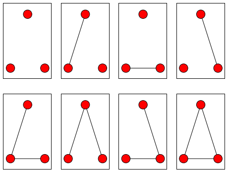
\[Pr(G)=\frac{exp(a∗edges(G)+b∗triangles(G))}{∑_{g∈G}exp(a∗edges(g)+b∗triangles(g))}\]Now we come to the first problem: calculating the denominator of that equation. There are many possible graphs. To take the simplest example, an undirected graph with 3 nodes has 8 possible configurations:
There are 64 possible configurations for a 4-node graph, and the number of possible configurations grows mind-bogglingly quickly after that. Most of the time, we simply can’t calculate the weights for all possible graphs. Instead, we need some sort of approximation.
We could just generate some large number of random graphs, and use that – but we have no way of knowing how representative they are of the actual distribution. We need a way to generate a sample that we think covers the most probable area of the distribution. In terms of the equation above, we want to sample heavily from networks where the weights are large, and less where the weights are small, so that the sum of the weights of the sample gets as close as possible to the actual total weight. Which brings us to the next step:
Markov Chain Monte Carlo
Markov Chain Monte Carlo (MCMC) actually refers a broad class of techniques for generating samples from complicated distributions. For our purposes, it means exploring the space of possible networks, moving toward the ones which are more likely given the distribution coefficients.
We’ll implement a simple version of the Metropolis-Hastings algorithm. We start with some network, and randomly add or subtract an edge.
def permute_graph(G):
    '''
    Return a new graph with an edge randomly added or subtracted from G
    '''
    G1 = nx.copy.deepcopy(G)
    d = nx.density(G1)
    r = random.random()
    if (r < 0.5 or d == 0) and d != 1:
        # Add an edge
        nodes = G.nodes()
        n1 = random.choice(nodes)
        n2 = random.choice(nodes)
        G1.add_edge(n1, n2)
    else:
        # Remove an edge
        n1, n2 = random.choice(G1.edges())
        G1.remove_edge(n1, n2)
    return G1
After the change, we check the weight on this new network.
- If it’s greater than the previous network’s weight (that is, it’s more probable under this distribution), we accept it and add it to our sample; it is also our new ‘current’ network.
- Otherwise, we might still accept it, deciding randomly based on the ratio between the new and old weights.
We repeat this many times, until we decide we have enough samples. The starting network can be any graph – I found that a random network worked well for my relatively small sample sizes, but we can also use the observed network itself, or a completely empty one. In theory, it shouldn’t matter after enough iterations.
def mcmc(G, edge_coeff, triangle_coeff, n):
    '''
    Use MCMC to generate a sample of networks from an ERG distribution.

    Args:
        G: The observed network, to seed the graph with
        edge_coeff: The coefficient on the number of edges
        triangle_coeff: The coefficient on number of triangles
        n: The number of samples to generate
    Returns:
        A list of graph objects
    '''

    v = len(G) # number of nodes in G
    p = nx.density(G) # Probability of a random edge existing
    current_graph = nx.erdos_renyi_graph(v, p) # Random graph
    current_w = compute_weight(G, edge_coeff, triangle_coeff)
    graphs = []
    while len(graphs) < n:
        new_graph = permute_graph(current_graph)
        new_w = compute_weight(new_graph, edge_coeff, triangle_coeff)
        if new_w > current_w or random.random() < (new_w/current_w):
            graphs.append(new_graph)
            current_w = new_w
    return graphs
So this code lets us generate a sample of networks from an exponential random graph distribution when we know the coefficients.
However, what we really want to do is find the coefficients. To do this, we want to look for the coefficients that describe an ERG distribution that makes the observed graph as likely as possible.
Fitting the model
The first thing we need to do is calculate the probability of observing any given graph, which means summing the weights of all the graphs in a sample:
def sum_weights(graphs, edge_coeff, tri_coeff):
    '''
    Sum the probability weights on every graph in graphs
    '''
    total = 0.0
    for g in graphs:
        total += compute_weight(g, edge_coeff, tri_coeff)
    return total
With this, we can calculate the probability of a given graph by dividing its weight by the sum of all weights from the sample.
Next, we can use our favorite optimization technique to hunt through the space of possible edge and triangle coefficients.
Instead of changing the network, we’ll randomly change the parameters, and use our MCMC function to estimate the probability of getting the observed network at those parameter values.
One simple way to do it uses a similar Metropolis-Hastings approach to the one we used above, with one tweak: early on, we want to try larger jumps around the parameter space; as we get further along, and hopefully closer to the ‘best’ value, the jumps should get smaller and smaller. There’s not really a right way to tweak the jump size
Here’s the code I came up with to do it:
def fit_ergm(G, coeff_samples=100, graph_samples=1000, return_all=False):
    '''
    Use MCMC to sample possible coefficients, and return the best fits.

    Args:
        G: The observed graph to fit
        coeff_samples: The number of coefficient combinations to sample
        graph_samples: The number of graphs to sample for each set of coeffs
        return_all: If True, return all sampled values. Otherwise, only best.
    Returns:
        If return_all=False, returns a tuple of values,
            (best_edge_coeff, best_triangle_coeff, best_p)
        where p is the estimated probability of observing the graph G with
        the fitted parameters.

        Otherwise, return a tuple of lists:
            (edge_coeffs, triangle_coeffs, probs)
    '''
    edge_coeffs = [0]
    triangle_coeffs = [0]
    probs = [None]

    while len(probs) < coeff_samples:
        # Make the jump size larger early on, and smaller toward the end
        w = coeff_samples/50.0
        s = np.sqrt(w/len(probs))
        # Pick new coefficients to try:
        edge_coeff = edge_coeffs[-1] +  random.normalvariate(0, s)
        triangle_coeff = triangle_coeffs[-1] + random.normalvariate(0, s)
        # Check how likely the observed graph is under this distribution:
        graphs = mcmc(G, edge_coeff, triangle_coeff, graph_samples)
        sum_weight = sum_weights(graphs, edge_coeff, triangle_coeff)
        p = compute_weight(G, edge_coeff, triangle_coeff) / sum_weight
        # Decide whether to accept the jump:
        if p > probs[-1] or random.random() < (p / probs[-1]):
            edge_coeffs.append(edge_coeff)
            triangle_coeffs.append(triangle_coeff)
            probs.append(p)
        else:
            edge_coeffs.append(edge_coeffs[-1])
            triangle_coeffs.append(triangle_coeffs[-1])
            probs.append(probs[1])
    # Return either the best values, or all of them:
    if not return_all:
        i = np.argmax(probs)
        best_p = probs[i]
        best_edge_coeff = edge_coeffs[i]
        best_triangle_coeff = triangle_coeffs[i]
        return (best_edge_coeff, best_triangle_coeff, best_p)
    else:
        return (edge_coeffs, triangle_coeffs, probs)
Example application
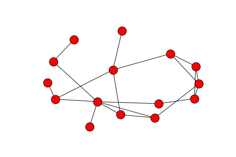
Now the real test – fitting the ERGM to an actual network. The canonical example is the Florentine marriage network, which is included in NetworkX.
G = nx.florentine_families_graph()
nx.draw(G)
%%timeit
graphs = mcmc(G, -1.25, 0.15, 10000)
1 loop, best of 3: 6.79 s per loop
I fit the ERGM with 100 coefficient iterations and 10,000 random networks for each candidate distribution. I also have it return the full series of steps. Note: this part takes a while.
%%timeit
edge_coeffs, triangle_coeffs, probs = fit_ergm(G, 10, 10, True)
The slowest run took 25.50 times longer than the fastest. This could mean that an intermediate result is being cached.
10 loops, best of 3: 199 ms per loop
edge_coeffs, triangle_coeffs, probs = fit_ergm(G, 100, 10, True)
i = np.argmax(probs)
print max(probs)
print edge_coeffs[i]
print triangle_coeffs[i]
0.59541550664
0.445701809562
-0.492293584485
Once it’s done (about 20 minutes later, for me), we can find the values it converged to. For me, they were:
Edge coefficient: -1.667
Triangle coefficient: -0.258
==========================
Summary of model fit
==========================

Formula:   flomarriage ~ edges + triangles

Iterations:  20

Monte Carlo MLE Results:
         Estimate Std. Error MCMC % p-value
edges     -1.6773     0.3499      0  <1e-04 ***
triangle   0.1574     0.5831      0   0.788
---
Signif. codes:  0 ‘***’ 0.001 ‘**’ 0.01 ‘*’ 0.05 ‘.’ 0.1 ‘ ’ 1
Not too far off! The edge coefficient is very close; the triangle coefficient is not too far off, and in any case isn't statistically significant.
One problem I discovered is that I obtained some estimated probabilities for the observed network that were greater than 1. This means that the network MCMC was sampling far away from the observed network, so that the weight on the observed network was greater than the sum of weights on all the sampled networks. This isn’t a great outcome, though it still does tell us something about how likely the observed network is under that distribution. Increasing the network sample size might help make this problem go away, as would improving the Markov chain procedure (e.g. with more permutation between networks).
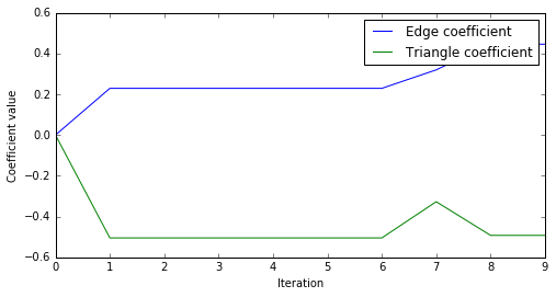
We can do a few more diagnostics on the results. For example, the trace of the value of the coefficients at each iteration is:
fig = plt.figure(figsize=(8,4))
ax = fig.add_subplot(111)
p1, = ax.plot(edge_coeffs)
p2, = ax.plot(triangle_coeffs)
ax.set_ylabel("Coefficient value")
ax.set_xlabel("Iteration")
l = ax.legend([p1, p2], ["Edge coefficient", "Triangle coefficient"])
weighted_edge_coeffs = np.array(edge_coeffs[1:]) * np.array(probs[1:])
print np.sum(weighted_edge_coeffs)/np.sum(probs[1:])
0.297715535504
weighted_tri_coeffs = np.array(triangle_coeffs[1:]) * np.array(probs[1:])
print np.sum(weighted_tri_coeffs)/np.sum(probs[1:])
-0.481915973737
We can also see the distribution of possible coefficients, by making a histogram weighted by the likelihood we observed for each value. (To deal with the likelihoods estimated at greater than 1, I actually weight each coefficient value by the log of the estimated likelihood).
fig = plt.figure(figsize=(12,4))
ax1 = fig.add_subplot(121)
ax1.hist(edge_coeffs[1:], weights=-np.log(probs[1:]))
ax1.set_title("Edge coefficient")
ax1.set_xlabel("Coefficient value")

ax2 = fig.add_subplot(122)
ax2.hist(triangle_coeffs[1:], weights=-np.log(probs[1:]))
ax2.set_title("Triangle coefficient")
ax2.set_xlabel("Coefficient value")
plt.show()
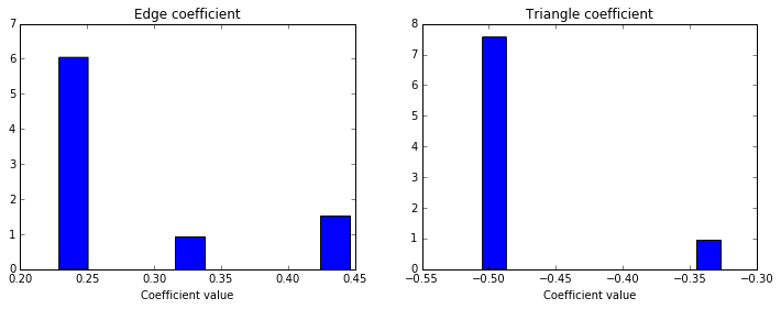
This shows that the bulk of the weight on the edge coefficient is between -1 and -2, while the triangle coefficient is much more evenly distributed on both sides of 0. Using a distribution like this, we can statistically test whether the coefficients are significantly different from 0, estimate the standard error, and do various other statistical tests and operations I won’t cover here.
And that’s it! We have a slow, simplistic but apparently somewhat-working ERGM model fitter, built up from scratch.
If you want to learn how to actually do ERGM analysis in R , Benjamin Lind has a great hands-on tutorial over at Bad Hessian on using ERGMs to model the hookup network on the TV show Grey’s Anatomy.
The paper introducing the ergm package by Hunter et al., the package developers, is a great guide
as is the (paywalled) An introduction to exponential random graph (p*) models for social networks by Robins et al.
Markov Chain Monte Carlo Estimation of Exponential Random Graph Models by Tom Snijders goes into more detail on estimation methodology, and includes an appendix with a much better estimation algorithm, which I may try to implement in the future.


Leave a Comment